Latent space
and control.

Instead of operating on raw pixels (which are heavy and slow), Stable Diffusion uses a Variational Autoencoder (VAE) to compress images 8× per side: a 512×512×3 image becomes a 64×64×4 latent — roughly 48× fewer numbers.

An important distinction: the SD VAE latent is a spatial compression code, not a map of meaning. Interpolating between two VAE latents gives ghostly pixel blends — not a dog smoothly morphing into a cat.

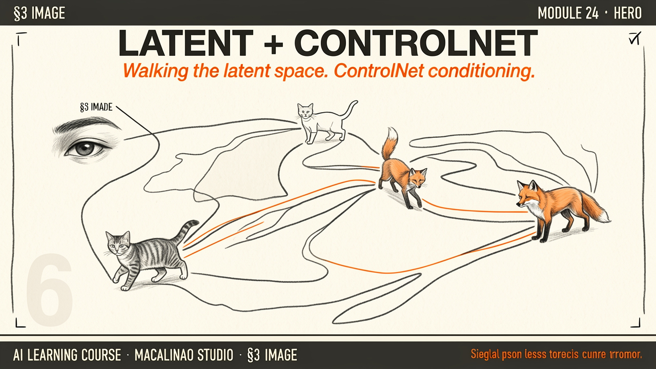
The famous dog→fox→cat smooth-interpolation story describes a semantic embedding space — a coordinate system where nearby points share meaning, like CLIP's text/image embedding space. Semantic interpolation in image generation happens in the text/conditioning space, or through the diffusion process itself — not by blending VAE latents. Keep the two spaces separate in your head: one stores where the pixels go, the other stores what the image means.

Imagine a tiny 2-dimensional semantic embedding space. The X-axis represents texture (Fluffy vs Scaley) and the Y-axis represents scale (Small vs Large). Drag your mouse around the grid to watch the corresponding image change! Note: this demo explores a conceptual embedding space — not the SD VAE's spatial compression latent.

While free generation is great for exploration, we often want specific compositions. ControlNet adds spatial conditioning: a trainable copy of the denoiser's encoder is attached to the frozen base model through zero-initialized convolutions, so training starts without disturbing it. Pass a stick-figure pose or a depth map and the copy injects that structure into generation. It is soft conditioning — outputs follow the structure closely but can deviate; nothing is mathematically locked.

These are often conflated. Flow matching / rectified flow is the incumbent training objective of 2026: learn a straight-line path from noise to image. FLUX-class models train this way — and still sample in 20–50 steps. Few-step generation (1–4 steps) comes from distillation: consistency models, LCM, DMD, and adversarial distillation compress a trained model's many sampling steps into a few.