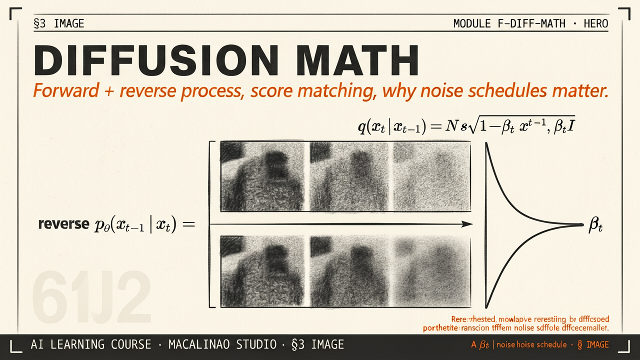
The forward process q(xt|xt-1) = N(xt; √(1-βt) xt-1, βt I) adds a small amount of Gaussian noise at each timestep. After T=1000 steps with a properly chosen noise schedule, the image is indistinguishable from pure Gaussian noise. The forward process has no learnable parameters — it's a fixed corruption schedule the model never has to predict.
REVERSE PROCESS
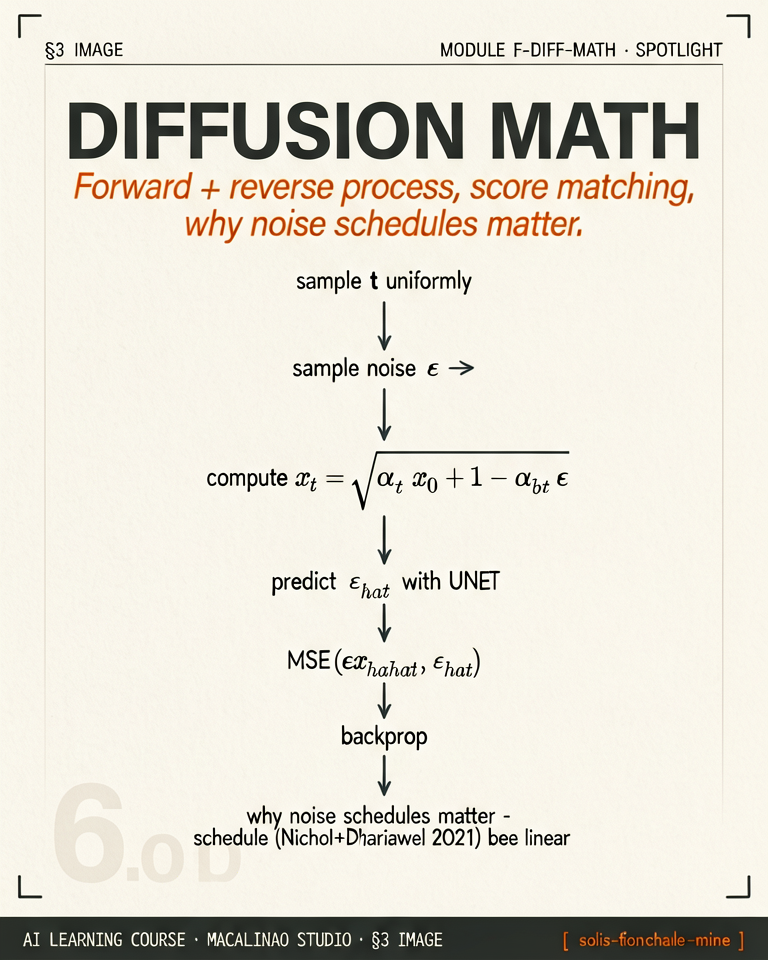
The model only has to learn one thing: predict the noise
The reverse process pθ(xt-1|xt) is what the network learns (historically a U-Net, today usually a diffusion transformer). At each timestep, given the noisy image xt, predict the noise ε that was added. Subtract a fraction of that prediction, get a slightly less noisy image xt-1. Repeat T times. The loss is simply L = ||ε - εθ(xt, t)||² — mean squared error between the true noise and the predicted noise.
SCORE MATCHING
Why noise prediction is equivalent to learning the data distribution
Song et al. (2021) showed that predicting noise is mathematically equivalent to estimating the score function∇x log p(x) — the gradient of the log-probability of the data distribution. Score matching is a well-studied technique going back to Hyvärinen 2005. Diffusion models are score-based models in disguise. This connection unifies DDPM with the earlier NCSN family of models.
NOISE SCHEDULE
Linear vs cosine vs sigmoid — the choice that affects everything
The schedule βt controls how fast information gets destroyed. The original DDPM paper used a linear schedule from β1=0.0001 to βT=0.02. iDDPM (Nichol & Dhariwal 2021) showed a cosine schedule preserves more signal in the early timesteps, leading to better samples. Modern systems use various variance-preserving / variance-exploding schedules. Practical takeaway: the schedule choice can change FID by several points.
FLOW MATCHING
Rectified flow — the objective behind FLUX/SD3-class models
Flow matching trains the network to predict a velocityv = x1 − x0 along a straight path from noise to data, with continuous time t ∈ [0,1] — replacing discrete β schedules entirely. Two practical companions: classifier-free guidance trains the model both with and without conditioning, then extrapolates between the two predictions at sampling time — the most-used equation in practice. And sampling takes 20–30 steps rather than 1000 because samplers like DDIM and DPM++ take larger, smarter steps along the learned trajectory.